Probabilistic Envelope for Delayed Teleoperation Under Environmental Uncertainty
Abstract
Delayed teleoperation requires operators to predict robot motion based on outdated feedback. This becomes especially challenging in environments such as the lunar surface, where uneven terrain and loose regolith create disturbances that make future robot states harder to estimate. Predictive displays help reduce the impact of communication delays by showing an estimate of the robot’s future state, allowing operators to anticipate what will happen after their inputs. However, most existing predictive displays either show a single predicted trajectory or only represent uncertainty using worst-case bounds. This can hide how likely different outcomes are, making it harder for operators to understand what the robot is most likely to do. In this paper, we introduce a Probabilistic Envelope, a visualization method that shows the most likely trajectory together with layered uncertainty bands. These bands use opacity to represent probability, making uncertainty easier to interpret. We evaluate the proposed method in a lunar rover simulation with a 2.56s communication delay. The results show that the Unscented Transform is more computationally efficient than the Monte Carlo method. In addition, the 1$\sigma$ and 2$\sigma$ uncertainty bands tend to overestimate environmental uncertainty, while the 3$\sigma$ band slightly underestimates it.
1 Introduction
Communication delays as small as 300 ms can already reduce the precision of robot control, and delays above 700 ms can make teleoperation extremely difficult or nearly impossible [1]. These delays are common in teleoperation, where humans control robots from a distance in hazardous or hard-to-reach environments such as collapsed buildings, dangerous industrial sites, and planetary exploration missions [2, 3]. In these situations, operators rely on remote sensing systems that are often limited by bandwidth, latency, and occlusions. Because of this, the feedback they receive about the robot and its environment is both delayed and incomplete.
In such settings, the normal feedback loop between action and observation is disrupted [4, 5]. Operators are forced to rely on outdated information, which reduces situational awareness and increases cognitive load [6, 7]. As a result, they often adopt a "move-and-wait" strategy, where the robot is advanced incrementally and then paused until feedback is received [4, 5, 8]. While this approach can reduce accumulated errors, it is inefficient and does not solve a key challenge: predicting robot motion under delay in uncertain environments.
This prediction problem becomes even more difficult in environments with strong variability. In such settings, the relationship between control commands and robot motion becomes difficult to infer [6, 4, 9]. This is particularly evident in planetary and lunar exploration, where communication delays are combined with loose regolith, uneven terrain, and changing traction conditions that cause unpredictable deviations in motion [10]. Studies on lunar rover mobility show that these terrain effects can significantly alter trajectories, making accurate prediction essential for safe and reliable operation [11]. As a result, operators must continuously estimate the robot’s state while accounting for both communication delay and environmental uncertainty, which is highly demanding under time pressure [12, 13, 14].
A common approach to address communication delay is the use of predictive displays. These interfaces estimate the robot’s near-future state so that operators can anticipate outcomes even when feedback is delayed [13, 15, 14]. A key challenge in these systems is how to represent uncertainty in a way that actually supports decision-making. Many existing methods rely on a single deterministic prediction, which hides important uncertainty caused by delays in command responses, imperfect control models, and environmental disturbances [14].
To address this, Cardinaels et al. [14] propose visualizations that explicitly show uncertainty in predictive displays. Their worst-case envelope extends the predicted trajectory into a cone-shaped region that captures possible deviations caused by disturbances. While this makes spatial uncertainty visible and can reduce cognitive load, it only represents the maximum possible error and treats all states within the envelope as equally likely. In other words, it shows where the robot might be, but not how likely each outcome is. Without this information, operators may find it harder to form an accurate mental model of future states [16, 17], potentially reducing trust in predictive displays and encouraging more reactive control strategies.
In this paper, we introduce a Probabilistic Envelope: a predictive visualization that represents both the expected future trajectory and the likelihood of deviations around it. We analytically approximate how uncertainty evolves by separating deterministic effects from zero‑mean, correlated ones. These modeled uncertainties are then communicated through a visual representation of layered confidence bands around a predicted mean trajectory over the delay horizon.
In short, we contribute:
- A decomposition of delayed teleoperation uncertainty into deterministic and correlated stochastic disturbance components relevant to predictive envelope generation.
- An analytical probabilistic modeling framework that propagates uncertainty using a combination of deterministic dynamics and correlated noise models, enabling real‑time prediction through the Unscented Transform.
- A Probabilistic Envelope visualization that externalizes these modeled uncertainties as layered confidence bands around a predicted mean trajectory.
- A technical evaluation demonstrating that the Probabilistic Envelope meets real‑time performance requirements and produces sigma‑level containment rates broadly consistent with theoretical expectations.
3 UNITE: A Lunar Robot Simulator
To develop and evaluate the Probabilistic Envelope, we rely on UNITE, a Unity‑based lunar robot simulation environment introduced by Cardinaels et al.[14]. UNITE provides a controlled simulation platform for studying delayed teleoperation, combining a configurable physics model with fixed communication delay and terrain‑dependent disturbances.
3.1 Robot Motion
UNITE simulates a TurtleBot3 Waffle Pi, a differential‑drive mobile robot whose motion follows the standard kinematic model. The operator provides discrete movement commands (forward, backward, left, right), which are translated by the simulator into left and right commanded wheel velocities, denoted \(v_{L}\) and \(v_R\). At each simulation step \(dt\), the simulator updates the robot’s pose and wheel velocities. For implementation purposes, UNITE stores the robot’s position \((x,y,z)\), heading \(\theta\), wheel velocities \((v_L,v_R)\), timestep \(dt\), and current input. The probabilistic model developed in this work primarily uses the planar pose \((x,z,\theta)\) and the wheel velocities \((v_L,v_R)\). The robot’s motion is determined by its linear and angular velocities. The linear velocity \(v\) is computed as the average of the wheel velocities: \[v = (v_L + v_R) / 2\] and the angular velocity \(\omega\) is computed from their difference, scaled by the robot’s wheelbase distance \(b\): \[\omega = (v_R - v_L) / b\] These velocities are then integrated over the timestep \(dt\) to update the robot’s pose: \[ x_{t+1} = x_t + v \cos(\theta_t)\, dt, \] \[ z_{t+1} = z_t - v \sin(\theta_t)\, dt, \] \[ \theta_{t+1} = \theta_t + \omega\, dt. \]
3.2 Communication Delay
To reproduce the temporal separation inherent to lunar teleoperation, UNITE incorporates a fixed one-way communication delay of 2.56 s. This value corresponds to the minimum signal propagation time between Earth and the Moon [21], thereby grounding the simulation in a realistic operational context.
In practice, the delay is implemented using a time‑stamped command queue. Each operator input is stored in this queue together with the simulation time at which it is scheduled to be executed. Rather than being applied immediately, commands are deferred until the full 2.56 s delay has elapsed.
During this waiting period, the queued inputs are also used to compute the predicted lookahead window. This ensures that the robot’s anticipated future trajectory is always derived from the same delayed command stream that governs its actual execution.
3.3 Environmental Disturbances
Beyond communication delay, UNITE incorporates a diverse set of environmental disturbances that reflect the variability encountered in planetary and lunar environments. These disturbances affect the robot’s wheel velocities before each kinematic update, causing deviations between commanded and executed motion. They include:
- Wheel Slip: Reduced traction on rough or loose surfaces lowers the effective wheel speeds, especially at higher velocities.
- Motor Variation: Time-dependent, deterministic variations in motor response independently modulate the left and right wheel velocities, introducing small but continuous asymmetries.
- Wheel Radius Variation: Slight differences in wheel radius introduce a slow, oscillatory turning tendency even under symmetric commands.
- Terrain Vibration: Spatially smooth terrain irregularities generate fluctuations in wheel motion.
- Encoder Noise: Additional variability is applied to wheel velocities to reflect imperfections.
- Slope Effects: Inclined terrain alters effective wheel velocities, causing downhill drift or resistance when moving uphill.
Disturbances (1) and (6) are directly governed by the terrain at the robot’s position. Wheel slip scales with both local surface roughness and the robot’s velocity, whereas slope effects are determined by the terrain gradient and the robot’s heading, introducing direction-dependent drift or resistance. Disturbances (2) and (3) are deterministic and time-dependent: motor variation is modeled through sinusoidal functions, while wheel-radius variation is represented by an anti-correlated sinusoidal signal applied to the left and right wheels. Disturbances (4) and (5) are derived from Perlin noise fields sampled at the robot’s location, generating spatially coherent vibration and encoder fluctuations that evolve smoothly as the robot traverses the environment. Although the resulting motion may appear irregular, all disturbance sources within UNITE’s physics model are deterministic, meaning that identical inputs consistently produce identical outcomes. This contrasts with stochastic uncertainty models, where disturbances are treated as random variables rather than fixed, repeatable dynamics.
To account for these environmental influences, the nominal wheel velocities \(v_{L}\) and \(v_R\), computed directly from operator input, are subsequently processed by the physics model. This yields modified wheel velocities that capture the combined effects of control input and terrain-dependent disturbances.
4 Probabilistic Modeling
A key challenge in delayed teleoperation is that operator commands are generated based on the robot’s currently observed state, but are only executed after a 2.56 s delay. During this time, the environment may change, and the robot can experience disturbances that could not be anticipated when the command was issued.
The Probabilistic Envelope is designed to help operators manage this uncertainty. It estimates how much the robot may deviate over the delay horizon. First, it computes a mean trajectory, which represents the most likely path of the robot given the queued commands and known deterministic effects of the environment. Around this mean, the method visualizes ±3$\sigma$ bands, which represent the expected range of deviations caused by temporally correlated noise over time.
To compute this envelope, we require a model that can capture uncertainty from environmental disturbances. A straightforward approach is Monte Carlo (MC) simulation, where the robot’s future motion is simulated multiple times while randomly sampling noise in each rollout. The resulting set of trajectories can then be used to approximate the distribution of future states. This approach is attractive because it does not assume a specific distribution shape and can therefore capture complex, non-Gaussian behavior.
However, in practice, this method is too computationally expensive for real-time use. Since the envelope must be updated continuously during operation, running a sufficient number of simulations to obtain stable estimates is not feasible. As shown empirically in Section 6.1, the required number of samples leads to unacceptable latency. For this reason, we instead use the Unscented Transform (UT), which provides an analytical approximation of uncertainty under the assumption that it follows a Gaussian distribution.
4.1 Modeling of Environmental Disturbances
To compute the mean trajectory and the corresponding sigma-bands, we separate disturbances in the physics model into two categories based on their characteristics.
Fully deterministic. As described in Section 3.3, we treat slip, motor variation, wheel radius variation, and slope bias as deterministic effects. These are modeled using functions whose future values are known exactly at the time of prediction. For instance, motor and wheel radius variations are represented as fixed-frequency sine waves that can be evaluated directly at any future timestep. The slope bias depends only on the terrain gradient and the rover’s heading, both of which are known in advance.
Slip is also treated as deterministic in this formulation. Given the current speed and terrain roughness, it produces a symmetric reduction in wheel speed that can be computed exactly. Since all of these effects can be determined for future timesteps without uncertainty, they are not treated as stochastic terms. Instead, they are directly incorporated into the mean wheel velocity.
Temporally correlated. The remaining disturbances, namely encoder noise and vibration noise, are treated as stochastic. As discussed in Section 3.3, they are modeled using Perlin noise fields, meaning their exact future values cannot be predicted. Unlike white noise, Perlin noise is smooth over time, so consecutive values are correlated rather than independent.
To model this temporal correlation in a tractable way, we use a first-order Gauss-Markov process. This is a natural choice because it captures temporal dependence through an exponentially decaying influence of past values.
4.2 Forward Propagation
At each update step, the mean trajectory and the sigma-bands are computed together in a single forward pass through the sequence of delayed control inputs. First, deterministic disturbances are applied to the commanded velocities to obtain the mean wheel velocities $\bar{v}_{L,k}$ and $\bar{v}_{R,k}$. These values are then propagated through the differential-drive kinematics to update the mean pose.
The sigma-bands require tracking how uncertainty evolves over the lookahead horizon. Because the differential-drive dynamics are nonlinear, linearization-based methods such as the Extended Kalman Filter can introduce errors that accumulate over time. Instead, the UT represents uncertainty using a small set of sample points. These points are propagated through the exact nonlinear motion model, and the resulting outputs are used to reconstruct the updated mean and covariance. This approach avoids linearization errors and provides a more accurate estimate of how uncertainty evolves over time, while still remaining computationally efficient.
Since vibration and encoder noise cannot be predicted exactly, their uncertainty must be propagated along with the kinematic state. For this reason, the four Gauss-Markov noise states are included directly in the state vector, resulting in a seven-dimensional representation: \[ \mathbf{x}_k = \bigl(x, z, \theta, n_{\text{vib},L}, n_{\text{vib},R}, n_{\text{enc},L}, n_{\text{enc},R}\bigr)_k. \]
This formulation allows the UT to propagate both pose and noise uncertainty in a single step, ensuring that the accumulated effect of temporally correlated disturbances is reflected in the sigma-bands as the prediction horizon increases.
We maintain a corresponding $7 \times 7$ covariance matrix $\Sigma_k$. At each step, it is propagated using the UT by first computing its Cholesky decomposition, which yields a lower-triangular matrix $L_k$ such that \[ \Sigma_k = L_k L_k^\top, \]
The columns of $L_k$ are then used to construct $2n = 14$ symmetric sigma points: \[ \mathcal{X}^{(i)}_k = \bar{\mathbf{x}}_k \pm \sqrt{n}\,(L_k)_i, \quad i = 1, \ldots, n, \] where $n = 7$ is the state dimension and $(L_k)_i$ denotes the $i$-th column of $L_k$.
The standard UT typically includes an additional sigma point at the mean, resulting in $2n+1$ points. In this work, we use a simplified parameterization with $\alpha = 1$ and $\kappa = 0$, which sets the scaling parameter $\lambda = \alpha^2(n+\kappa) - n$ to zero. With this choice, the central point has zero weight and is omitted, leaving $2n$ equally weighted points with $W_i = \tfrac{1}{2n}$.
Each sigma point is then propagated through the nonlinear differential-drive kinematics, and the updated covariance is reconstructed as \[ \Sigma_{k+1} = \sum_{i=1}^{2n} W_i \left(\mathcal{X}^{(i)}_{k+1} - \bar{\mathbf{x}}_{k+1}\right) \left(\mathcal{X}^{(i)}_{k+1} - \bar{\mathbf{x}}_{k+1}\right)^\top + Q_k, \]
The matrix $Q_k$ represents process noise added at each propagation step. It has two components. First, noise is injected into the vibration and encoder states to prevent their uncertainty from artificially shrinking over long horizons. Second, a residual pose-level noise term is included to capture effects not modeled in the deterministic dynamics, such as unmodeled slip and small terrain irregularities. This pose-level term is projected along the rover’s heading and wheelbase, preserving correlations between $x$, $z$, and $\theta$.
After obtaining \(\Sigma_{k+1}\), the lateral uncertainty \(\sigma_{\text{lat}}\) is computed by projecting the positional covariance onto the lateral direction vector \((\sin\theta_k,\ \cos\theta_k)^\top\): \[ \sigma_{\text{lat}} = \sqrt{\sin^2\theta_k\,\Sigma_{xx} + 2\sin\theta_k\cos\theta_k\,\Sigma_{xz} + \cos^2\theta_k\,\Sigma_{zz}}, \]
Finally, the \(\pm 1\sigma\), \(\pm 2\sigma\) and \(\pm 3\sigma\) bounds are constructed symmetrically around the mean trajectory along this lateral direction, forming the Probabilistic Envelope visualized during teleoperation.
5 Probabilistic Envelope Design
Building upon the probabilistic trajectory data described in the preceding section, the Probabilistic Envelope visualization is constructed as a layered, surface-aligned structure comprising a mean trajectory ribbon and up to three nested sigma-bands.
The mean trajectory represents the expected path over the lookahead horizon, while the sigma-bands capture the predicted spread of future robot states across that same horizon, mainly reflecting left and right deviations around the mean trajectory.
As illustrated in Figure 1, the sigma-bands are projected onto the lunar terrain geometry, ensuring spatial coherence between the predicted envelope and the underlying topography. The 1$\sigma$ band corresponds to the region of highest concentration of likely deviations, with the 2$\sigma$ and 3$\sigma$ bands encompassing progressively less probable, though still physically plausible, deviations.
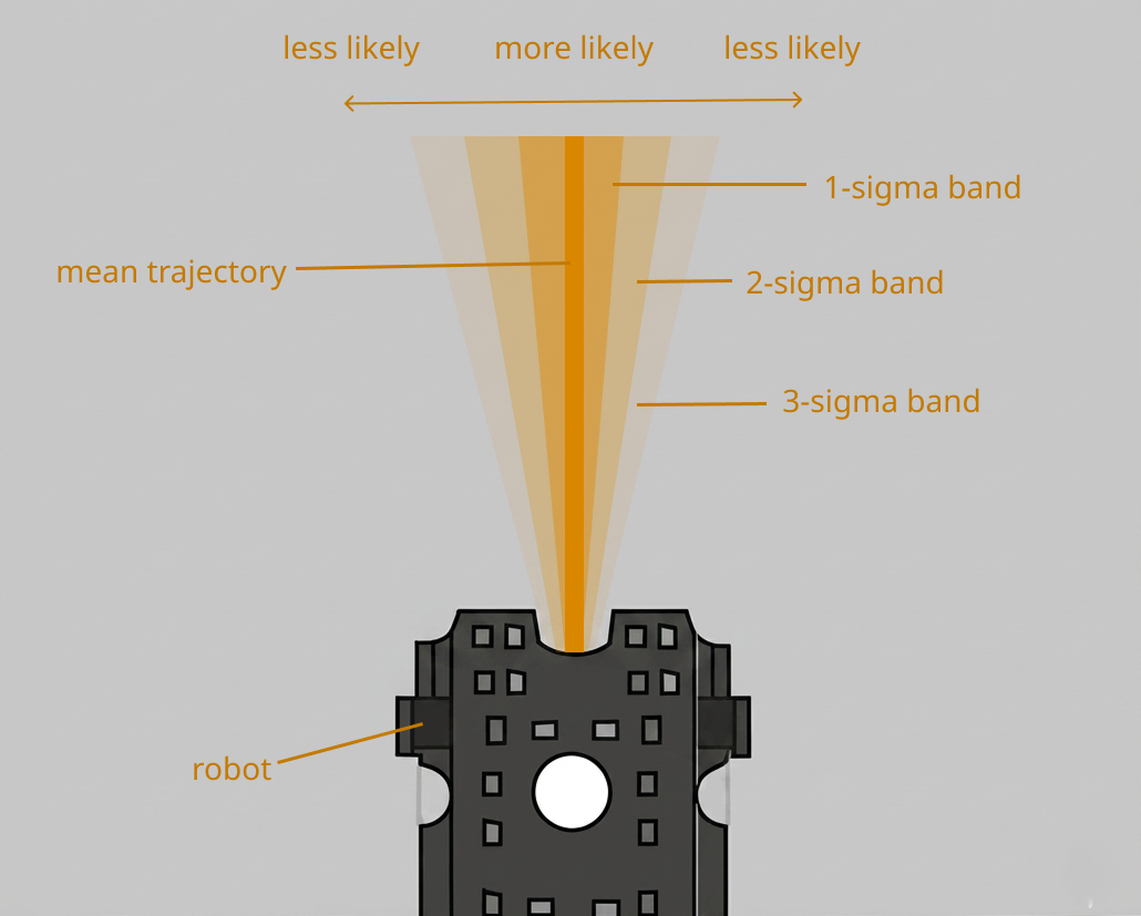
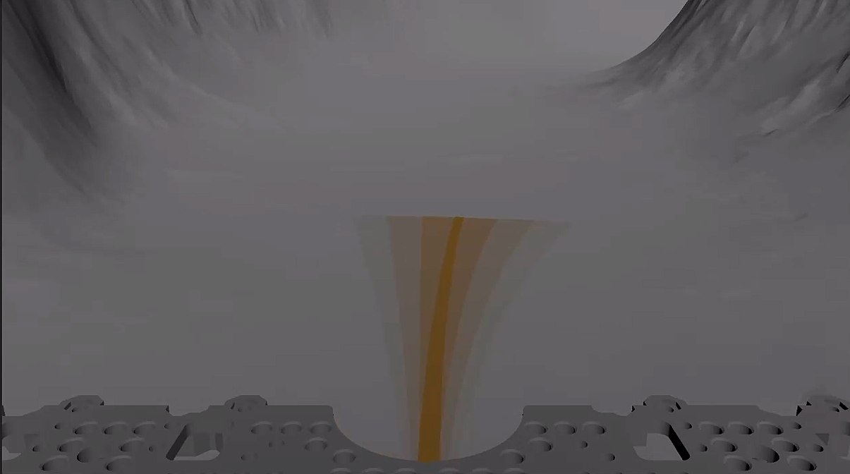
Likelihood is conveyed through two complementary visual cues: spatial proximity to the mean trajectory and opacity. Regions of higher opacity indicate higher probability density, while the decreasing opacity of the outer bands reflects lower-density, lower-likelihood deviations. The opacity-based encoding is motivated by Seipp et al. [34], who found that opacity-based encodings can support accurate interpretation of areal uncertainty, and by Correll et al. [35], who showed that reducing visual detail in high-uncertainty regions encourages more cautious decision-making. Together, these cues are intended to help operators assess both the expected motion and the degree of uncertainty along the predicted path.
As the operator maintains a forward velocity command, the Probabilistic Envelope extends dynamically across the full prediction horizon, up to the limit imposed by the fixed communication delay.
6 Technical Evaluation
To technically evaluate the proposed Probabilistic Envelope, we tested its computational performance and predictive calibration within the UNITE simulator. Because the primary goals of the envelope are to operate in real-time and to produce calibrated uncertainty bounds under simulated disturbances, our evaluation focuses on two metrics: (1) computational efficiency, and (2) predictive accuracy. All tests were conducted over a simulated 2.56 s communication delay, using a Lenovo ThinkBook 15 G3 ACL equipped with an AMD Ryzen 7 processor, 16 GB of RAM, and an AMD Radeon GPU, running Windows 11. Operator input was provided via a Logitech G413 TKL SE keyboard. The UNITE simulator was developed and executed in Unity 6000.0.45f1, running at a fixed physics update rate of 50 Hz and rendered at 120 FPS, with all commands streamed in real time subject to the imposed communication delay.
6.1 Computational Efficiency
The main motivation for adopting the Unscented Transform (UT) over Monte Carlo (MC) rollouts was real-time feasibility. MC was still included because it provides a straightforward way to model non-Gaussian uncertainty without relying on Gaussian assumptions. To evaluate both approaches, we benchmarked the execution time required to compute the lookahead envelope on a per-frame basis.
In the MC approach, the algorithm iterates over all inputs stored in the delayed command queue. For each input, a set of simulated trajectories is propagated forward in time. All samples start from the same initial state but evolve differently due to stochastic perturbations, which are decorrelated using unique Perlin-noise offsets per sample. This allows the method to avoid Gaussian assumptions and produce a trajectory distribution that better reflects the variability of the underlying dynamics.
At each prediction step, the lateral deviation of each sample is computed by projecting its displacement onto the lateral axis defined by the mean heading. These deviations are then sorted to form an empirical distribution, from which percentile-based bounds are extracted. The inner band corresponds to the 25th–75th percentiles (50% of samples), the middle band to the 5th–95th percentiles (90% of samples), and the outer band to the 1st–99th percentiles (98% of samples). These percentile offsets are then mapped back into spatial coordinates to construct the final envelope boundaries.
Both methods were evaluated under controlled conditions. The simulator generated predictions over 500 frames, each using a horizon of 128 input steps determined by the communication delay and the physics update rate. For the MC method, the computation was repeated with different numbers of samples to study how runtime scales with trajectory count.
The experiments were conducted under three physics profiles representing a lunar-like rough surface, a smooth flat surface, and loose sand. Each profile captures a different operating regime relevant to off-road rover dynamics. The parameter configurations are listed in Table 1.
| Parameter | Moon | Flat Surface | Loose Sand |
|---|---|---|---|
| Roughness | 0.7 | 0.2 | 0.5 |
| Wheel slip | 0.15 | 0.1 | 0.35 |
| Motor response variation | 0.05 | 0.02 | 0.08 |
| Wheel radius variation | 0.02 | 0.01 | 0.05 |
| Encoder noise | 0.04 | 0.005 | 0.06 |
| Vibration intensity | 0.08 | 0.02 | 0.05 |
| Vibration frequency | 3 Hz | 1 Hz | 2 Hz |
Figures 2 and 3 compare elapsed time across physics profiles and methods. The red dashed line indicates the 8.33 ms per-frame budget at 120 FPS, which must accommodate rendering, physics, input handling, and envelope computation. Exceeding this budget by the envelope alone makes frame drops unavoidable, while staying below it does not guarantee real-time performance due to other Unity overhead.
The UT method averages 800 µs per frame across all physics profiles, whereas MC ranges from 10 ms (100 samples) to 63 ms (550 samples), exceeding the frame budget in all configurations. UT remains below the threshold in nearly all cases, with only three outliers slightly above it.
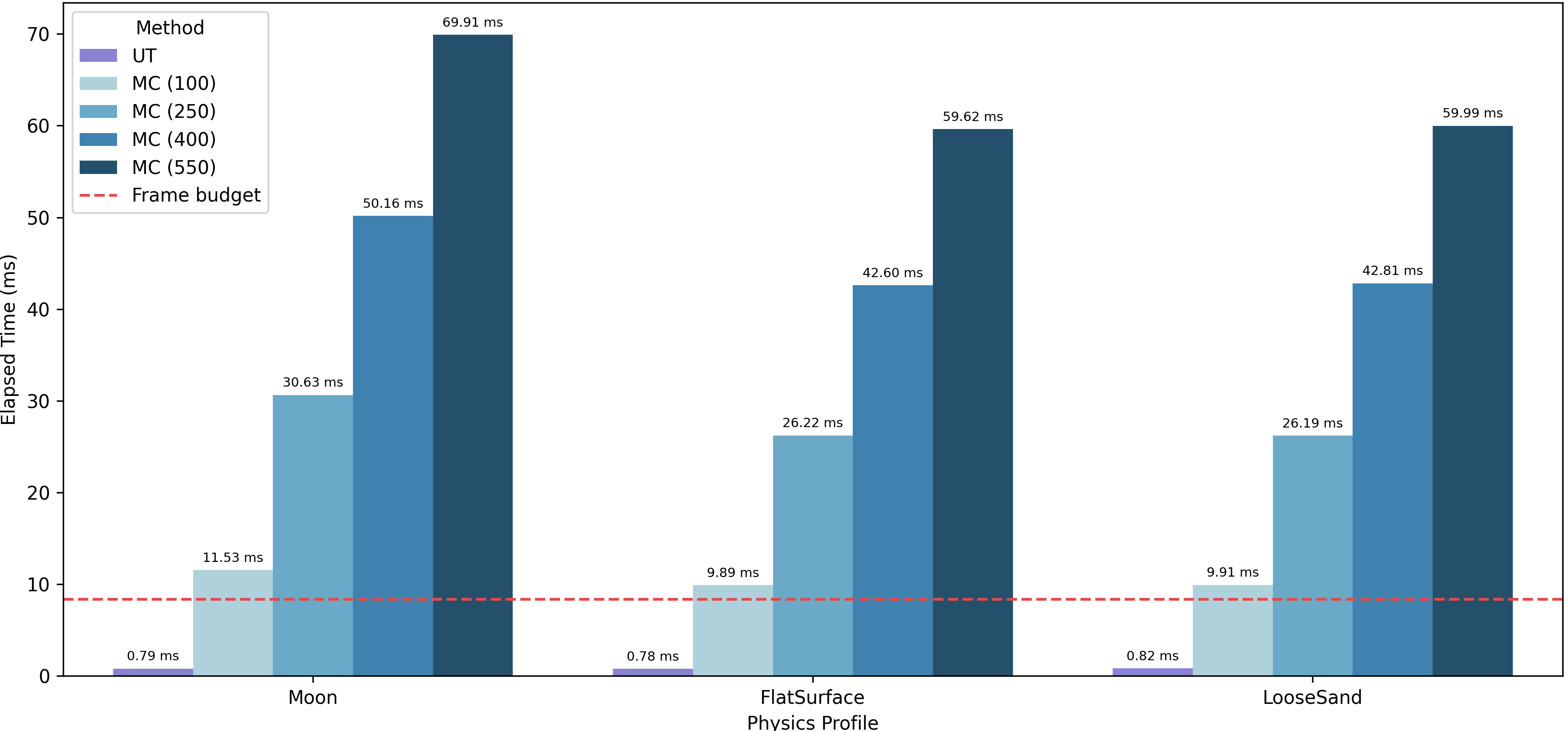
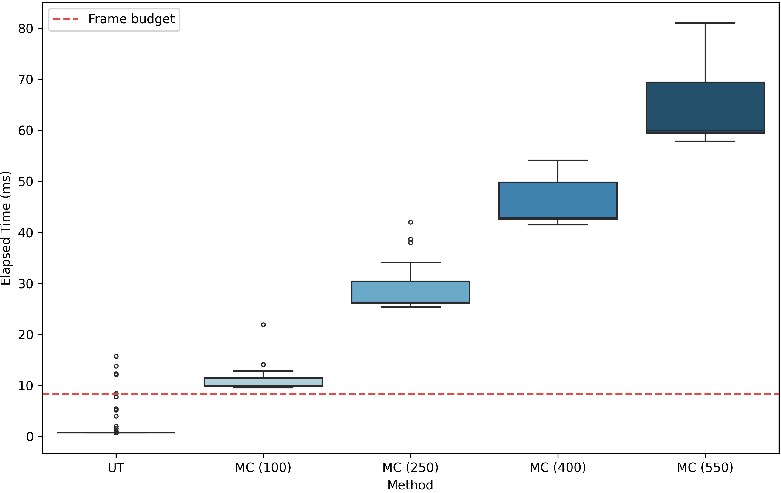
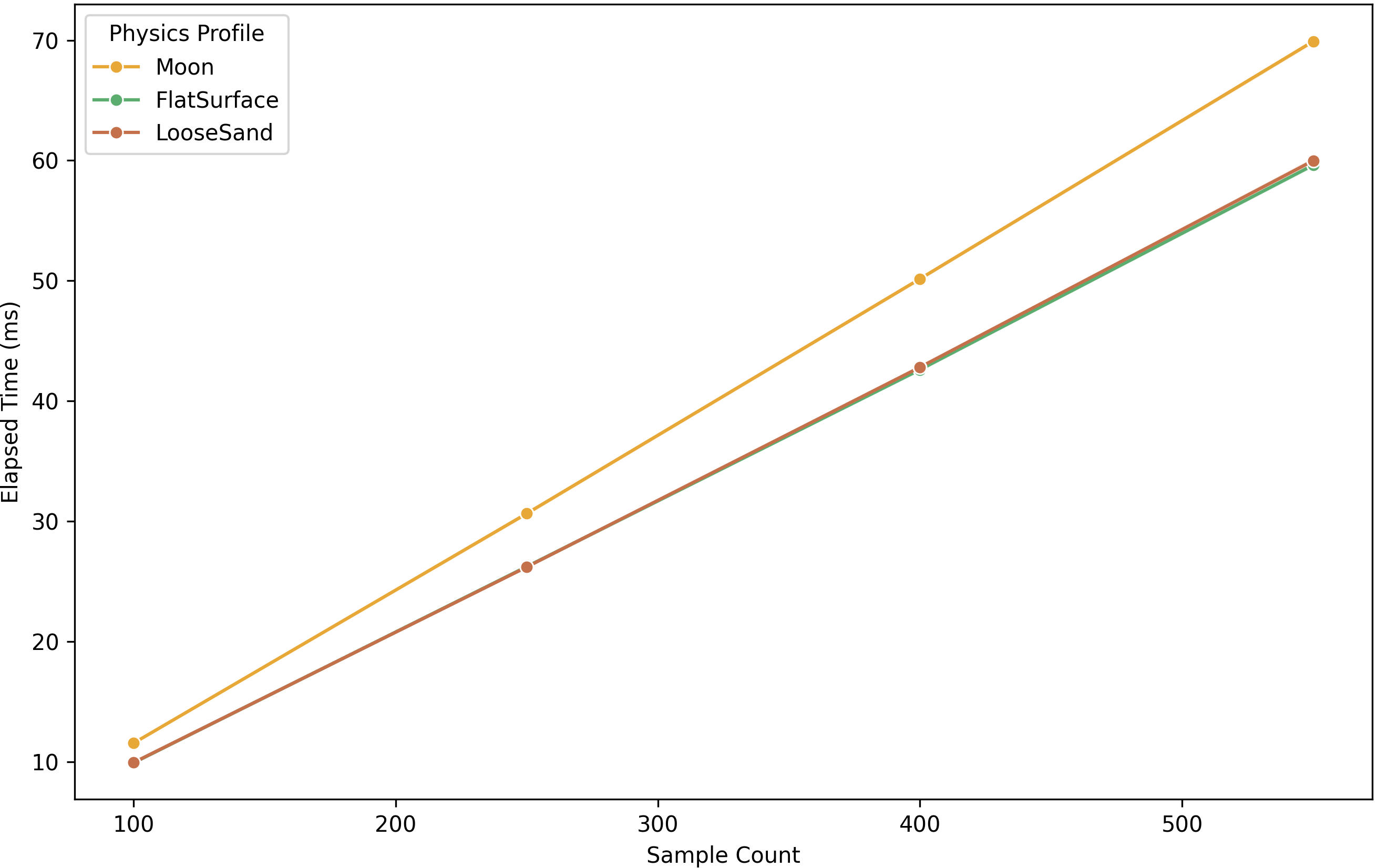
Figure 4 shows that elapsed time scales linearly with sample count across all physics profiles. The Moon profile incurs a consistently higher cost than FlatSurface and LooseSand, a difference that grows from approximately 1.5 ms at 100 samples to 10 ms at 550 samples.
6.2 Predictive Calibration and Containment
To verify that the predicted uncertainty envelopes accurately reflect the physical disturbances present in the simulator, we evaluate the containment rate of the Probabilistic Envelope. If the probabilistic model is well calibrated, the robot’s actual trajectory should fall within the $1\sigma$ boundary approximately 68% of the time, within the $2\sigma$ boundary approximately 95%, and within the $3\sigma$ boundary approximately 99.7% of the time, consistent with the expected containment probabilities of a Gaussian distribution.
To evaluate containment, three quantities were logged at each simulation frame. First, the robot’s actual position in world space. Second, the predicted mean trajectory produced at that frame, storing the expected $(x, z)$ position for each step in the prediction horizon alongside the originating frame index and the corresponding target frame index. Finally, the left and right boundary points of the $1\sigma$, $2\sigma$, and $3\sigma$ sigma-bands were recorded for each horizon step as $(x, z)$ pairs, each associated with its from-frame and target-frame indices.
The experiment used the moon physics preset designed to reproduce key disturbance characteristics of low-gravity, irregular terrain. The corresponding physics parameters are listed in Table 2.
| Parameter | Value |
|---|---|
| Roughness | 0.7 |
| Wheel slip | 0.15 |
| Motor response variation | 0.05 |
| Wheel radius variation | 0.02 |
| Encoder noise | 0.04 |
| Vibration intensity | 0.08 |
| Vibration frequency | 3 Hz |
The robot was driven manually along a single constrained path, since the terrain geometry allowed no alternative routes. The trajectory covered 15.05 m over 167.8 s.
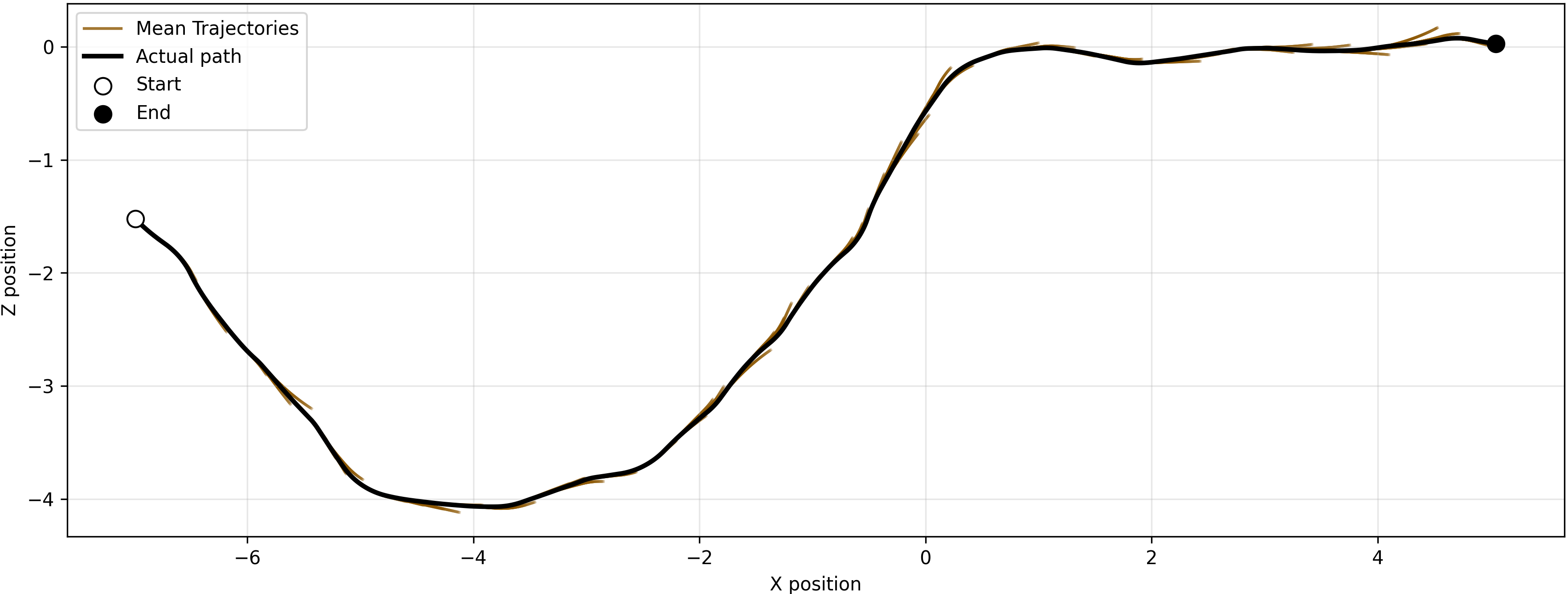
The predictive behavior of the mean trajectory is illustrated in Figure 5(a). At each frame, the model generates a full forward prediction from the robot’s current state independently, without using any temporal memory of previous predictions. To keep the visualization readable, 100 frames are uniformly sampled from the recorded sequence.
For each sampled frame, the predicted mean positions over the horizon are connected to form a short trajectory segment starting from the robot’s actual position at that frame. When placed along the full trajectory, these segments show how the model’s predictions evolve as new observations become available. Segments that closely follow the actual trajectory indicate accurate mean predictions, while segments that deviate highlight regions where prediction reliability decreases. As shown in Figure 5(a), the predicted segments remain closely aligned with the robot’s trajectory throughout the run.
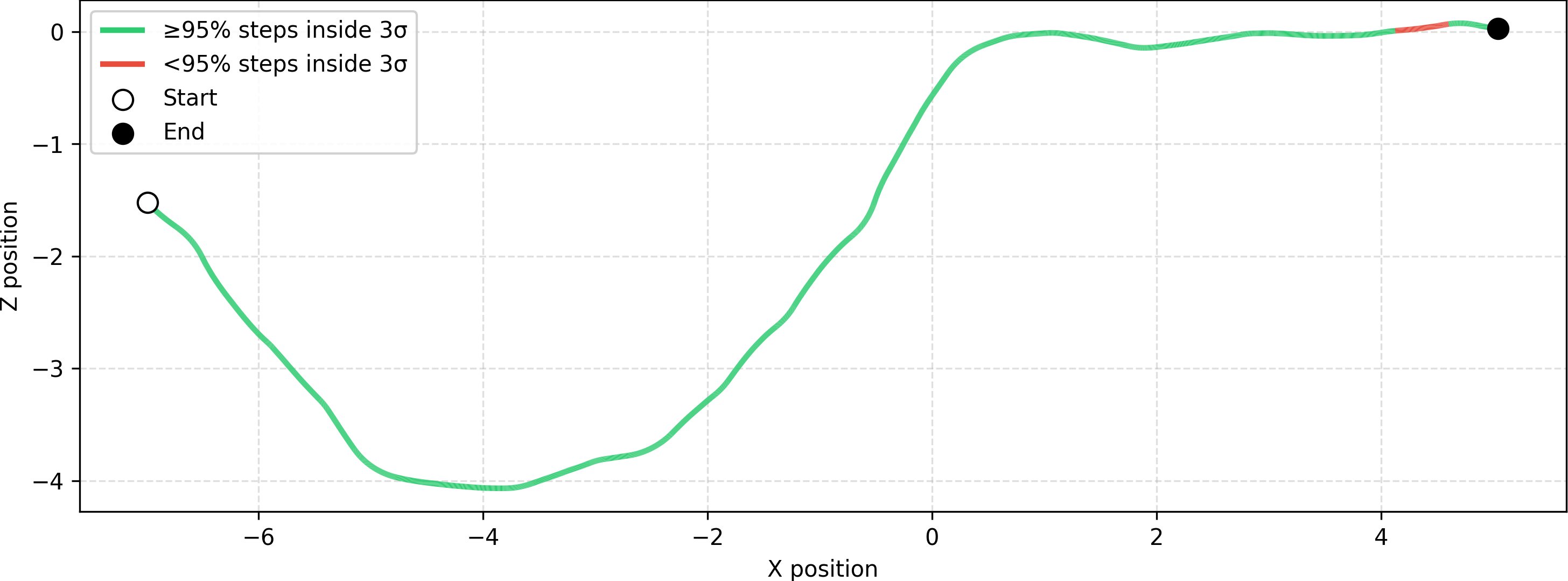
While the mean trajectory captures expected motion, it does not provide information about uncertainty. Figure 5(b) therefore evaluates whether the robot’s actual position lies within the $3\sigma$ bounds of the Probabilistic Envelope at each frame. For each prediction, a lateral containment test is performed: the robot’s actual position is projected onto the lateral axis defined by the predicted mean and the left $1\sigma$ boundary, producing a signed lateral displacement relative to the predicted mean.
A frame is marked green if at least 95% of the predictions reaching that frame contain the robot within the corresponding $3\sigma$ lateral interval, and red otherwise. As shown in Figure 5(b), the trajectory is mostly green, with a short red section near the end of the run.
To quantify these results, Table 3 reports containment rates for the $1\sigma$, $2\sigma$, and $3\sigma$ bands. Since a new prediction is generated at every frame and each prediction spans multiple future horizon steps, the evaluation produces a large number of prediction-observation pairs obtained by merging actual positions, mean predictions, and sigma envelopes across matching frame–horizon indices. For each pair, the robot’s actual future position is expressed relative to the predicted mean and projected onto a locally defined lateral axis derived from the $1\sigma$ boundary geometry. The containment test is then performed by computing the signed lateral offset of the actual position with respect to the mean and checking whether it lies between the projected left and right sigma bounds for each confidence level. The containment rate is computed as the fraction of pairs where this offset lies within the corresponding $1\sigma$, $2\sigma$, and $3\sigma$ intervals.
| Sigma | Result | Expected |
|---|---|---|
| 1$\sigma$ | 80.41% | 68% |
| 2$\sigma$ | 97.69% | 95% |
| 3$\sigma$ | 99.28% | 99.7% |
The $1\sigma$ and $2\sigma$ containment rates exceed their theoretical Gaussian expectations, with observed rates of 80.41% against an expected 68.27% for $1\sigma$, and 97.69% against an expected 95.45% for $2\sigma$. The $3\sigma$ containment rate of 99.28% falls marginally below the theoretical value of 99.73%.
7 Discussion and Future Work
The computational performance results show that the UT is significantly more efficient for real-time use. On average, UT is 9.2 ms faster than the MC method at 100 samples, and 62.2 ms faster at 550 samples. While these differences may seem small in isolation, they become important when compared to the 8.33 ms frame budget required for 120 frames per second.
The MC method requires a relatively large number of samples to produce a sufficiently expressive approximation of the probability distribution. However, its computational cost increases linearly with the number of samples, as shown in Figure 4. This creates a clear trade-off: increasing the sample count improves the quality of the uncertainty representation, but makes real-time performance difficult or impossible to achieve.
In addition, the physics profile affects computation time. The lunar profile is consistently the most expensive due to higher terrain roughness, which triggers additional noise-related computations. In contrast, the smooth and sandy profiles show lower and more similar runtimes.
The containment analysis shows an overestimation at the 1$\sigma$ and 2$\sigma$ bands, but a slight underestimation at the 3$\sigma$ band, which is consistent with Figure 5(b), which shows the robot leaving the 3$\sigma$ band at the end of the trajectory. The overestimation at the inner bands occurs because the UT accumulates process noise additively at every prediction step, causing the predicted bands to grow wider and wider the further ahead you look. The actual robot is physically constrained and cannot deviate arbitrarily far from the mean path, so in practice the true spread grows more slowly than the model predicts. This means more actual positions fall inside the inner bands than a Gaussian would expect. The underestimation at 3$\sigma$ has a different cause. In the simulation, noise is applied multiplicatively to the wheel velocities. This could occasionally produce sudden large deviations that are larger than the model would estimate.
The 3$\sigma$ band escape seen at the end of the trajectory occur because the rover was driven closer to steep terrain edges during that portion of the experiment run, causing larger deviations than those encountered during the rest of the run. The probabilistic envelope, was unable to capture this more rare worst-case scenario.
The containment analysis shows that the uncertainty is overestimated at the $1\sigma$ and $2\sigma$ levels, but slightly underestimated at the $3\sigma$ level. This is consistent with Figure 5(b), which shows the robot leaving the $3\sigma$ envelope near the end of the trajectory.
The overestimation in the inner bands can be explained by a mismatch between the uncertainty model used by the UT and the actual robot dynamics. The UT propagates sigma points through the motion model without considering physical limits. In contrast, the simulated robot clamps wheel velocities to a maximum value at every timestep, representing the physical limits of the motors. As a result, disturbances that would cause wheel speeds to exceed this limit are effectively absorbed by the clamp and do not affect the robot’s motion. The UT, however, still considers these larger deviations possible, causing it to predict a wider spread of trajectories than is observed in practice.
The slight underestimation at the $3\sigma$ level has a different cause. In the simulation, noise is applied multiplicatively to the wheel velocities, which can occasionally produce large deviations that are not fully captured by the Gaussian approximation. These rare events can lead to outcomes beyond the $3\sigma$ bound.
This effect is particularly visible near the end of the experiment in Figure 5(b), where the rover is driven closer to steep terrain edges than during the rest of the run. This leads to larger-than-usual deviations, causing the robot to leave the $3\sigma$ envelope. As a result, the probabilistic envelope does not fully capture these rare worst-case conditions.
The mean trajectory also demonstrates strong predictive accuracy. As shown in Figure 5(a), the predicted mean path remains closely aligned with the robot’s actual trajectory throughout the experiment. In some regions, the predicted segments do not perfectly match the robot’s subsequent motion. One possible explanation is that the operator used the predictive information to make corrective steering adjustments during teleoperation. Since the mean trajectory indicates the robot’s most likely future motion, deviations caused by environmental disturbances become visible before they occur. This allows the operator to anticipate drift and apply corrective inputs, helping keep the robot closer to the intended path.
Several limitations should be acknowledged. First, the evaluation was conducted entirely within the UNITE simulation environment. Although the simulator includes realistic communication delays and terrain-dependent disturbances, simulated physics cannot fully capture the variability, sensor noise, and mechanical interactions present in real-world robotic systems.
In addition, this work does not include a human-subject evaluation. While the Probabilistic Envelope was designed to improve the communication of uncertainty and support operator decision-making, its effect on operator performance has not yet been experimentally validated. In particular, it remains unclear how the visualization influences situational awareness, trust, cognitive workload, and overall task performance during delayed teleoperation. It is also unknown how operators would use and interpret the visualization during extended or high-pressure tasks.
These limitations provide several directions for future work. Most importantly, the proposed visualization should be evaluated through controlled user studies to determine its impact on operator behavior, decision-making, cognitive workload, and task performance under communication delay. In addition, future research should investigate how the method performs on physical robotic platforms, where real-world disturbances and sensing imperfections may affect the accuracy of the predicted uncertainty bounds.
Conclusion
The challenges of delayed teleoperation extend beyond the communication delay itself. Operators must also deal with uncertainty caused by environmental variability, which makes it more difficult to predict the robot’s future state. In this work, we investigated how communication delays and environmental disturbances affect the prediction of future robot motion. To address this problem, the different sources of uncertainty were separated into deterministic and temporally correlated components, allowing their effects to be modeled and propagated over the prediction horizon.
Based on this framework, the Probabilistic Envelope was developed to visualize future robot states as a probability distribution rather than a single trajectory or worst-case bound. The visualization displays the predicted mean trajectory together with sigma-bands that represent the expected growth of uncertainty over time. The inner bands indicate the most likely deviations, while the outer bands capture less likely but still plausible deviations.
The evaluation showed that the Unscented Transform provides a computationally efficient way to generate these predictions in real time. The predicted mean trajectory remained closely aligned with the robot’s actual path throughout the experiment, demonstrating good predictive accuracy. The results also showed that the uncertainty bounds tend to overestimate the spread of the robot’s motion at the $1\sigma$ and $2\sigma$ levels, while slightly underestimating it at the $3\sigma$ level. Overall, the findings suggest that the proposed approach can effectively communicate the expected trajectory while remaining suitable for real-time teleoperation, despite a tendency to overestimate uncertainty.
Beyond the technical outcomes, the development of the Probabilistic Envelope proved to be a demanding process due to limited existing knowledge on applying probability theory in robotics, as well as challenges in modeling physics in general. These constraints made it difficult to identify a method that was both appropriate and computationally efficient for representing environmental uncertainty in a probabilistic manner. While the approach ultimately adopted may not be the most optimal, it nevertheless serves as an initial step toward communicating uncertainty to the operator in a probabilistic form.
Acknowledgments
I would like to thank my supervisors, Dries Cardinaels and Prof. dr. Kris Luyten for their guidance and support throughout this individual project. I am also grateful that I had the chance to use the UNITE simulation environment, for the development and evaluation of this individual project.
AI usage
During this individual project, I made use of Claude and ChatGPT to improve the writing and readability of the text. They were also used during the implementation phase to search for implementation approaches and to understand how certain aspects could be implemented, such as the probabilistic modeling.
The code was always checked afterwards and modified if necessary. Generated output was never directly adopted without review. I always evaluated the suggestions, adapted them where needed, and rejected them when appropriate.
References
- S. B. Kamtam, Q. Lu, F. Bouali, O. C. L. Haas, and S. Birrell. 2024. Network Latency in Teleoperation of Connected and Autonomous Vehicles: A Review of Trends, Challenges, and Mitigation Strategies. Sensors 24, 12 (2024), 3957. https://doi.org/10.3390/s24123957
- D. W. Hainsworth. 2001. Teleoperation User Interfaces for Mining Robotics. Autonomous Robots 11, 1 (2001), 19–28. https://doi.org/10.1023/A:1011299910904
- R. R. Murphy. 2004. Activities of the rescue robots at the World Trade Center from 11–21 September 2001. IEEE Robotics & Automation Magazine 11, 3 (2004), 50–61. https://doi.org/10.1109/MRA.2004.1337826
- William R. Ferrell. 1965. Remote manipulation with transmission delay. IEEE Transactions on Human Factors in Electronics HFE-6, 1 (1965), 24–32. https://doi.org/10.1109/THFE.1965.6591253
- William R. Ferrell and Thomas B. Sheridan. 1967. Supervisory control of remote manipulation. IEEE Spectrum 4, 10 (1967), 81–88.
- Zhaokun Chen, Wenshuo Wang, Wenzhuo Liu, Yichen Liu, and Junqiang Xi. 2025. The Effects of Communication Delay on Human Performance and Neurocognitive Responses in Mobile Robot Teleoperation.
- Euijung Yang and Michael C. Dorneich. 2017. The Emotional, Cognitive, Physiological, and Performance Effects of Variable Time Delay in Robotic Teleoperation. International Journal of Social Robotics 9, 4 (2017), 491–508. https://doi.org/10.1007/s12369-017-0407-x
- Miran Seo, Samraat Gupta, and Youngjib Ham. 2024. Exploratory study on time-delayed excavator teleoperation in virtual lunar construction simulation: Task performance and operator behavior. Automation in Construction 168 (2024), 105871. https://doi.org/10.1016/j.autcon.2024.105871
- Parinaz Farajiparvar, Hao Ying, and Abhilash Pandya. 2020. A Brief Survey of Telerobotic Time Delay Mitigation. Frontiers in Robotics and AI 7. https://doi.org/10.3389/frobt.2020.578805
- Daniel Lester and Harley Thronson. 2011. Low-latency lunar surface telerobotics from Earth-Moon libration points. In AIAA Space 2011 Conference & Exposition. 7341.
- Mark Allan, Uland Wong, P. Michael Furlong, Arno Rogg, Scott McMichael, Terry Welsh, Ian Chen, Steven Peters, Brian Gerkey, Morgan Quigley, Mark Shirley, Matthew Deans, Howard Cannon, and Terry Fong. 2019. Planetary Rover Simulation for Lunar Exploration Missions. In 2019 IEEE Aerospace Conference. 1–19. https://doi.org/10.1109/AERO.2019.8741780
- Henrikke Dybvik, Martin Lland, Achim Gerstenberg, Kristoffer Bjrnerud Slttsveen, and Martin Steinert. 2021. A low-cost predictive display for teleoperation: Investigating effects on human performance and workload. International Journal of Human-Computer Studies 145 (2021), 102536. https://doi.org/10.1016/j.ijhcs.2020.102536
- A. K. Bejczy, W. S. Kim, and S. C. Venema. 1990. The phantom robot: predictive displays for teleoperation with time delay. In Proceedings of the IEEE International Conference on Robotics and Automation. 546–551. https://doi.org/10.1109/ROBOT.1990.126037
- Dries Cardinaels, Raf Ramakers, Tom Veuskens, Thomas Pietrzak, Gustavo Alberto Rovelo Ruiz, and Kris Luyten. 2026. Every Move You Make: Visualizing Near-Future Motion Under Delay for Telerobotics. In Proceedings of the 2026 CHI Conference on Human Factors in Computing Systems. Association for Computing Machinery, New York, NY, USA, https://doi.org/10.1145/3772318.3791452
- A. K. Bejczy and Won S. Kim. 1990. Predictive displays and shared compliance control for time-delayed telemanipulation. In IEEE International Workshop on Intelligent Robots and Systems, Towards a New Frontier of Applications. 407–412. https://doi.org/10.1109/IROS.1990.262418
- Mica R. Endsley. 1995. Toward a Theory of Situation Awareness in Dynamic Systems. Human Factors: The Journal of the Human Factors and Ergonomics Society 37, 1 (1995), 32–64. https://doi.org/10.1518/001872095779049543
- Mark Colley, Christian Bräuner, Mirjam Lanzer, Marcel Walch, Martin Baumann, and Enrico Rukzio. 2020. Effect of Visualization of Pedestrian Intention Recognition on Trust and Cognitive Load. In 12th International Conference on Automotive User Interfaces and Interactive Vehicular Applications. Association for Computing Machinery, New York, NY, USA, 181–191. https://doi.org/10.1145/3409120.3410648
- Kyohei Otsu, Guillaume Matheron, Sourish Ghosh, Olivier Toupet, and Masahiro Ono. 2020. Fast approximate clearance evaluation for rovers with articulated suspension systems. Journal of Field Robotics 37 (2020), 768–785. https://doi.org/10.48550/arXiv.1808.00031
- J. Borenstein and Liqiang Feng. 1996. Measurement and correction of systematic odometry errors in mobile robots. IEEE Transactions on Robotics and Automation 12, 6 (1996), 869–880. https://doi.org/10.1109/70.544770
- Sebastian Thrun, Wolfram Burgard, and Dieter Fox. 2005. Probabilistic Robotics. MIT Press, Cambridge, MA.
- NASA Glenn Research Center. 2000. Seeing the Earth, Seeing the Moon (Earth–Moon–Earth Communication). Accessed: 2025-08-21. https://www.grc.nasa.gov/www/k12/Numbers/Math/Mathematical_Thinking/seeing_the_earth_moon.htm
- A. Trivedi, M. Zolotas, A. Abbas, S. Prajapati, S. Bazzi, and T. Padr. 2024. A Probabilistic Motion Model for Skid-Steer Wheeled Mobile Robot Navigation on Off-Road Terrains. In 2024 IEEE International Conference on Robotics and Automation (ICRA). 12599–12605. https://doi.org/10.1109/ICRA57147.2024.10611343
- C. Cunningham, M. Ono, I. Nesnas, J. Yen, and W. L. Whittaker. 2017. Locally-adaptive slip prediction for planetary rovers using Gaussian processes. In Proceedings of the IEEE International Conference on Robotics and Automation (ICRA). 5487–5494. https://doi.org/10.1109/ICRA.2017.7989646
- Barnali Das and Gordon Dobie. 2021. Delay compensated state estimation for Telepresence robot navigation. Robotics and Autonomous Systems 146 (2021), 103890. https://doi.org/10.1016/j.robot.2021.103890
- Daniel Szafir and Danielle Albers Szafir. 2021. Connecting Human-Robot Interaction and Data Visualization. In Proceedings of the 2021 ACM/IEEE International Conference on Human-Robot Interaction. Association for Computing Machinery, New York, NY, USA, 281–292. https://doi.org/10.1145/3434073.3444683
- Matthew Kay, Tara Kola, Jessica R. Hullman, and Sean A. Munson. 2016. When (ish) is My Bus? User-centered Visualizations of Uncertainty in Everyday, Mobile Predictive Systems. In Proceedings of the 2016 CHI Conference on Human Factors in Computing Systems. Association for Computing Machinery, New York, NY, USA, 5092–5103. https://doi.org/10.1145/2858036.2858558
- Miriam Greis, Jessica Hullman, Michael Correll, Matthew Kay, and Orit Shaer. 2017. Designing for Uncertainty in HCI: When Does Uncertainty Help? In Proceedings of the 2017 CHI Conference Extended Abstracts on Human Factors in Computing Systems. Association for Computing Machinery, New York, NY, USA, 593–600. https://doi.org/10.1145/3027063.3027091
- J. Hullman, X. Qiao, M. Correll, A. Kale, and M. Kay. 2019. In Pursuit of Error: A Survey of Uncertainty Visualization Evaluation. IEEE Transactions on Visualization and Computer Graphics 25, 1 (2019), 903–913. https://doi.org/10.1109/TVCG.2018.2864889
- L. Padilla, M. Kay, and J. Hullman. 2026. Uncertainty Visualization. In Wiley StatsRef: Statistics Reference Online, N. Balakrishnan and T. Colton and B. Everitt and W. Piegorsch and F. Ruggeri and J. L. Teugels (Ed.). Wiley, https://doi.org/10.1002/9781118445112.stat08296
- Alex Pang, Craig Wittenbrink, and Suresh Lodha. 1997. Approaches to uncertainty visualization. The Visual Computer 13 (1997), 370–390. https://doi.org/10.1007/s003710050111
- C. Olston and J. D. Mackinlay. 2002. Visualizing data with bounded uncertainty. In IEEE Symposium on Information Visualization 2002 (INFOVIS 2002). 37–40. https://doi.org/10.1109/INFVIS.2002.1173145
- Daniel Weiskopf. 2022. Uncertainty Visualization: Concepts, Methods, and Applications in Biological Data Visualization. Frontiers in Bioinformatics 2 (2022), 793819. https://doi.org/10.3389/fbinf.2022.793819
- T. Gschwandtner, M. Bögl, P. Federico, and S. Miksch. 2016. Visual Encodings of Temporal Uncertainty: A Comparative User Study. IEEE Transactions on Visualization and Computer Graphics 22, 1 (2016), 539–548. https://doi.org/10.1109/TVCG.2015.2467752
- Karsten Seipp, Francisco Guti\’errez, Xavier Ochoa, and Katrien Verbert. 2019. Towards a visual guide for communicating uncertainty in Visual Analytics. Journal of Computer Languages 50 (2019), 1–18. https://doi.org/10.1016/j.jvlc.2018.11.004
- Michael Correll, Dominik Moritz, and Jeffrey Heer. 2018. Value-Suppressing Uncertainty Palettes. In Proceedings of the 2018 CHI Conference on Human Factors in Computing Systems. Association for Computing Machinery, New York, NY, USA, https://doi.org/10.1145/3173574.3174216
- Mark Colley, Oliver Speidel, Jan Strohbeck, Jan Ole Rixen, Jan Henry Belz, and Enrico Rukzio. 2023. Effects of Uncertain Trajectory Prediction Visualization in Highly Automated Vehicles on Trust, Situation Awareness, and Cognitive Load. Proc. ACM Interact. Mob. Wearable Ubiquitous Technol. 7, 4. https://doi.org/10.1145/3631408
- L. E. Matzen, B. C. Howell, M. C. S. Trumbo, and K. M. Divis. 2023. Numerical and Visual Representations of Uncertainty Lead to Different Patterns of Decision Making. IEEE Computer Graphics and Applications 43, 5 (2023), 72–82. https://doi.org/10.1109/MCG.2023.3299875
- Nadia Boukhelifa and David John Duke. 2009. Uncertainty visualization: why might it fail? In CHI ’09 Extended Abstracts on Human Factors in Computing Systems. Association for Computing Machinery, New York, NY, USA, 4051–4056. https://doi.org/10.1145/1520340.1520616
- Melanie Bancilhon, Zhengliang Liu, and Alvitta Ottley. 2019. Let’s Gamble: Uncovering the Impact of Visualization on Risk Perception and Decision-Making. https://doi.org/10.48550/arXiv.1910.09725
- A. M. van der Bles, S. van der Linden, A. L. J. Freeman, and D. J. Spiegelhalter. 2020. The effects of communicating uncertainty on public trust in facts and numbers. Proceedings of the National Academy of Sciences 117, 14 (2020), 7672–7683. https://doi.org/10.1073/pnas.1913678117
- J. Reyes, A. U. Batmaz, and M. Kersten-Oertel. 2025. Trusting AI: does uncertainty visualization affect decision-making? Frontiers in Computer Science 7 (2025), 1464348. https://doi.org/10.3389/fcomp.2025.1464348